Conditional Formatting in Excel with Copilot

I don’t pretend to be an Excel genius, but over time I have developed some tips and tricks that I use to make my life easier. One thing that I do when I am reviewing an M365 tenant is to populate an Excel workbook with the current settings of the tenant. At some point I am going to get the M365DSC to do this for me…but that is in the future.

What I have right now in the various tabs of the workbooks are a series of columns that list the location of the setting in the UI, and then I have populated a column that displays the Microsoft Default value for that setting. The next two columns are then populated with the Current Value in the tenant and then the Recommended Value.

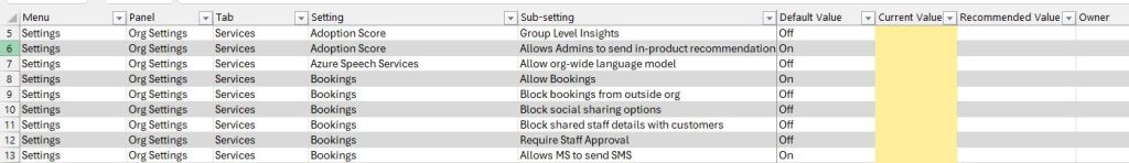
Once I have this populated, what I would love to have happen is for the Current Value to be highlighted if it is different from the Default Value, and the same to be true of the Recommended Value if it varies from the Current Value. I used to do this by hand because I never could see how to do it using the Conditional Formatting menu options.

Enter Copilot. I asked Copilot to highlight the cells in the Current Value if it was different from the Default Value and it came back with a quick and easy resolution. The trick is to use the New Rule Menu and then to select the “Use a formula to determine which cells to format” option. This allows us to use the following formula to do a comparative highlighting of the cells. You could use it to highlight ones that match or don’t or pretty much anything. The formula that Copilot suggested was:

$G2 <> $F2

When applied to the G column (or at least the G column in my table), if it is different from the F column (Default Value) then it will be highlighted (in this case with a manila-colored background. I then did the same with the Recommended Value column to mark it as Green if it is different, although I suppose what I should do is mark it Green when it matches the Current Value to show that there is no change. Either way works.

Create your Conditional Formatting Formula

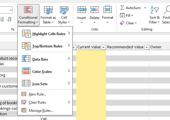
Step 1: Select the range of cells that you want to format (column G in my example)

Step 2: Open up the Conditional Formatting Menu and select New Rule (third from the bottom)

Step 3: In the New Formatting Rule Pop-Up, Select the bottom Type “Use a formula to determine which cells to format”

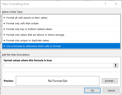
Step 4: In the Formula use an Absolute Column “$” and a relative row for each side ($G2<>$F2) in my initial example.

Step 4: Click on the Format button and set the cell to be whatever you need it to be. For me, I set the Fill to RGB 255,239,156 which gave me a nice manilla color, and I left the text Black. For the second one I used Dark Green for the Text color, and Light Green for the Fill.

Step 5: Click on OK twice to accept the Format and the Rule and then voila.

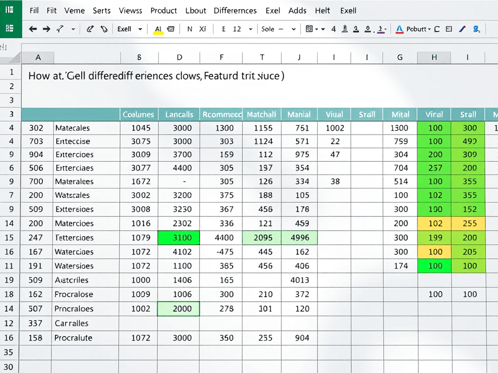
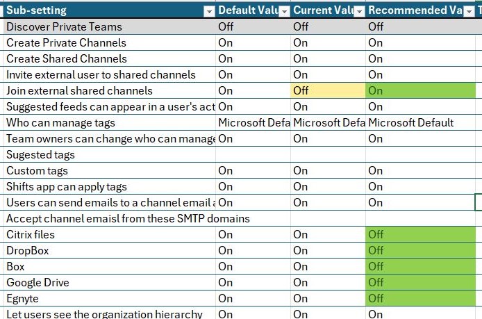
The final product looks like this:

I hope that this explanation on how to do this fairly simple task that I had never figured out until I asked Copilot makes your life easier. I think it demonstrates how Copilot is changing the way that we look for solutions. I used to have to search the web or Excel help for this type of thing and if you didn’t know the right words to use for the features it got almost impossible. With Copilot I told it what I wanted, and it figured out how to do the search and told me how to solve my problem.